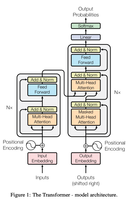
Transformer

Transformers are a type of deep learning model that revolutionized natural language processing (NLP) and other fields like computer vision. Introduced in the paper “Attention is All You Need” by Vaswani et al. in 2017, Transformers leverage self-attention mechanisms to process and generate data more efficiently than previous models like RNNs and LSTMs. They excel at handling sequential data, enabling breakthroughs in tasks such as machine translation, text generation, and even image recognition. The architecture’s scalability and versatility have made it a foundational tool in modern AI research and applications.

In this post, I’ll focus mainly on two main component of the Transformer architecture

• The Multi-head Self-Attention mechanism
• Position-wise Feed-Forward Network

Multi-head Self Attention

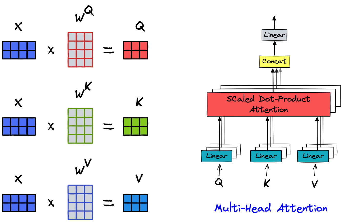
Multi-head attention is a core component of the Transformer architecture. The idea behind multi-head attention is to allow the model to focus on different parts of the input sequence from multiple perspectives simultaneously. This is achieved by using multiple attention heads, each of which computes scaled dot-product attention independently. Given an input sequence represented by a matrix $X\in {\mathbb{R}}^{n\times d}$, where $n$ is the sequence length and $d$ is the dimensionality of each input vector, multi-head attention is computed as follows:

1. Linear Projections: The input $X$ is linearly projected into queries, keys, and values using learned weight matrices $W_Q$, $W_K$, and $W_V$ respectively:

$$Q=X{W}_Q,K=X{W}_K,V=X{W}_V$$

2. Scaled Dot-Product Attention: Each attention head computes the scaled dot-product attention:

$$\text{Attention}(Q,K,V)=\text{softmax}\left(\frac{Q{K}^{\top }}{\sqrt{d_k}}\right)V$$

where $d_k$ is the dimensionality of the keys (or queries), and the scaling factor $\frac{1}{\sqrt{d_k}}$ helps to stabilize the gradients.

4. Multi-Head Attention: The outputs from each attention head are concatenated and linearly transformed using a weight matrix $W_O$:

$$\text{MultiHead}(Q,K,V)=\text{Concat}({\text{head}}_1,{\text{head}}_2,\dots ,{\text{head}}_h)W_O$$

where ${\text{head}}_i=\text{Attention}(Q_i,K_i,V_i)$, and $h$ is the number of attention heads. By using multiple heads, the model can capture different aspects of the input data, leading to richer representations and better performance on various tasks.

Position-wise Feed-Forward Network

In the Transformer architecture, the Position-wise Feed-Forward Network (FFN) is applied independently to each position in the sequence. It provides additional non-linearity and depth to the model. The FFN is composed of two linear transformations with a ReLU activation in between. Given an input $x\in {\mathbb{R}}^d$, where $d$ is the dimensionality of the input, the FFN can be defined as: $\text{FFN}(x)=\text{max}(0,x{W}_1+b_1)W_2+b_2$ Here:

• $W_1\in {\mathbb{R}}^{d\times d_{ff}}$ and $W_2\in {\mathbb{R}}^{d_{ff}\times d}$ are learned weight matrices,
• $b_1\in {\mathbb{R}}^{d_{ff}}$ and $b_2\in {\mathbb{R}}^d$ are bias terms,
• $d_{ff}$ is the dimensionality of the hidden layer, typically larger than $d$,
• $\text{max}(0,x)$ represents the ReLU activation function.

The Position-wise FFN is applied to each position in the sequence separately and identically. Despite its simplicity, the FFN contributes significantly to the Transformer’s ability to model complex patterns in the data. In architectures for Large Language Models with billions of parameters, the hidden size $d$ typically has very large values.

Model	no Layers	No heads	$d$	LR	Batch
125M	12	12	768	6.0e-4	0.5M
350M	24	16	1024	3.0e-4	0.5M
1.3B	24	32	2048	2.0e-4	1M
2.7B	32	32	2560	1.6e-4	1M
6.7B	32	32	4096	1.2e-4	2M
13B	40	40	5120	1.0e-4	4M
30B	48	56	7168	1.0e-4	4M
66B	64	72	9216	0.8e-4	2M
175B	96	96	12288	1.2e-4	2M

Other components

Apart from the two main components mentioned above, the Transformer’s strength also inherits several powerful features from previous architectures. These include the ability to handle sequential data like RNN-based models (using position embeddings), solving limitations, such as vanishing/exploding gradients (Layer Norm, Residual Connection).

Embedding Layer

The input tokens (words or subwords) are first converted into dense vectors (embeddings) that capture their meanings in a continuous space. These embeddings are learned during training or set fixed depending on the choice of the author.

Positional Embeddings

Since the Transformer architecture processes all tokens in parallel, it’s essential to inject positional information into each token. This is where positional embeddings become crucial.

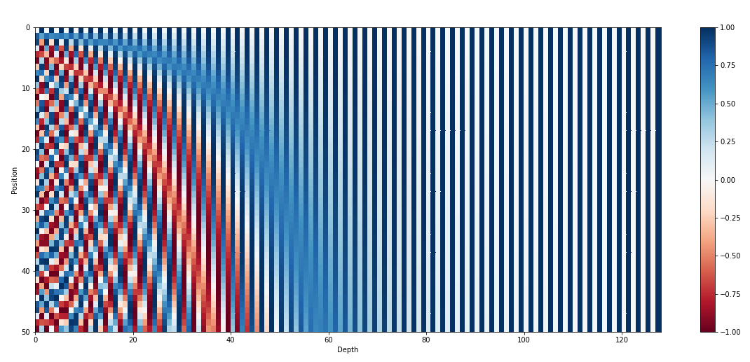
The positional encodings are defined using sine and cosine functions of different frequencies. For a given position $pos$ and dimension $i$, the positional encoding is computed as:

$$PE(pos,2i)=\sin \left(\frac{pos}{10000^{\frac{2i}{d_{\text{model}}}}}\right)$$ $$PE(pos,2i+1)=\cos \left(\frac{pos}{10000^{\frac{2i}{d_{\text{model}}}}}\right)$$

Where

• $pos$ is the position of the token in the sequence (e.g., 1st, 2nd, 3rd, etc.).
• $i$ is the dimension index within the embedding.
• $d_{\text{model}}$ is the dimensionality of the model (i.e., the size of the embedding vectors).

note

• Different Frequencies for Each Dimension: Sine functions are used for even dimensions and cosine functions for odd dimensions, with varying frequencies, uniquely encoding each position while maintaining smoothness.
• Smooth Changes Across Positions: The smooth variation in sine and cosine functions ensures that small position changes lead to small encoding changes, providing relative positioning.
• Additive to Embeddings: Positional encodings are added to token embeddings, merging positional and semantic information.

This is the positional encoding implementation that is used in the original Transformer paper, however in recent Large Language Model variants, a more popular type of positional encoding is Relative Positional Encoding

Layer Normalization

Layer Norm is applied after the attention mechanism and the feed-forward network to stabilize and speed up training. It normalizes the outputs of these layers, ensuring that the model can learn effectively.

note

In the original paper, the authors used Layer Norm right after MSA and FFN blocks (post norm), however it is proved that used Layer Norm before MSA and FFN (pre norm) lead to more stable training.

Residual Connections

To help the model retain information from earlier layers, Residual Connection are added around the self-attention and feed-forward layers. These connections allow the model to learn the difference between the input and output of each layer, making training easier and improving performance.